Loss Functions Part 2
In this part of the multi-part series on the loss functions we'll be taking a look at MSE, MAE, Huber Loss, Hinge Loss, and Triplet Loss. We'll also look at the code for these Loss functions in PyTorch and some examples of how to use them


- Mean Squared Error
- Mean Absolute Error Loss (MAE)
- Huber Loss
- Hinge Loss
- Triplet Loss
- Summary
- References
import torch
from torch import nn
from torch.autograd import Variable
import numpy as np
from matplotlib import pyplot as plt
precision=4
np.set_printoptions(precision=precision)
In this post, I'd like to ensure that we're able to code the loss classes ourselves as well, that means that we'll need to be able to:
- Translate the equations to Python code for
forwardpass. - Know how to calculate the gradients for a few loss functions, so that when we call
backwardpass the gradients get accumulated.
Note that in presence of autodiff or autograd we won't need to do such a thing and this is purely for learning perspective, better implementations are offered by Deep Learning Libraries like PyTorch, Tensorflow etc.
So, we'll define a class called Module that we'll use and override its forward and backward abstract functions
from abc import ABC, abstractmethod

class Module(ABC):
    def __init__(self, reduction='mean'):
        self.grad_input = None
        self.reduction = reduction

    def __call__(self, input, target):
        return self.forward(input, target)

    @abstractmethod
    def forward(*args, **kwargs):
        pass

    @abstractmethod
    def backward(*args, **kwargs):
        pass

    def update_grad_input(self, grad):
        if self.grad_input is not None:
            self.grad_input += grad
        else:
            self.grad_input = grad

    def zero_grad(self):
        if self.grad_input is not None:
            self.grad_input = np.zeros_like(self.grad_input)
After having setup our base class, we can now look at individual Loss functions and start coding them.
Mean Squared Error
Mean Squared Error (MSE) measures the average of the squares of the errors for an estimator. The MSE of an estimator $\hat{\theta}$ wrt an unknown parameter $\theta$ is defined as $MSE(\hat{\theta}) =E[(\hat{\theta} - \theta)^2]$. It can also be written as the sum of Variance and the squared Bias of the estimator. In case of an unbiased estimator the MSE and variance are equivalent. Below is a quick way to see how the MSE and the Variance and Bias are related to each other.
using the following result:
We arrive at:
We can see from above that as Variance, MSE also heavily weights the outliers. It's squaring each term which weights large error terms more heavily than smaller ones. An alternative in that becomes Mean Absolute Error which is the topic of discussion of next section.
class MSELoss(Module):
    def __init__(self, reduction='mean'):
        super(MSELoss, self).__init__(reduction)

    def forward(self, input, target):
        if self.reduction is not None:
            red = getattr(np, self.reduction)
        else:
            red = np.asarray
        return np.asarray([red((target-input)**2),])

    def backward(self, input, target):
        N = np.multiply.reduce(input.shape)
        grad = (2/N * (input-target))
        self.update_grad_input(grad)
Forward pass using our Implementation
reduction = 'mean'
SEED=42
rs = np.random.RandomState(SEED)
input = rs.randn(3,2,4,5)
target = rs.randn(3,2,4,5)

mse = MSELoss(reduction)
loss = mse(input, target)
loss
Let's test our implementation against PyTorch and see if we've implemented things correctly or not.
Using the same input and target numpy.ndarray as torch.tensor
Forward pass using PyTorch's Implementation
criterion = nn.MSELoss(reduction=reduction)
inp = Variable(torch.from_numpy(input), requires_grad=True)
loss = criterion(inp, torch.from_numpy(target))
loss
Comparing gradients
loss.backward()
mse.backward(input, target)
np.allclose(mse.grad_input, inp.grad.numpy())
As pointed out earlier the MSE Loss suffers in the presence of outliers and heavily weights them. MAE on the other hand is more robust in that scenario. It is defined as the average of the absolute differences between the predictions and the target values.
$$ MAE(\hat{\theta}) = (E[|\hat{\theta} - \theta|]) $$It is also knows as the L1Loss as it is measuring the L1 distance between two vectors
class L1Loss(Module):
    def __init__(self, reduction='mean'):
        super(L1Loss, self).__init__(reduction)

    def forward(self, input, target):
        if self.reduction is not None:
            red = getattr(np, self.reduction)
        else:
            red = np.asarray
        return np.asarray([red((np.abs(target-input))),])

    def backward(self, input, target):
        N = np.multiply.reduce(input.shape)
        diff = input - target
        mask_lg = (diff > 0) * 1.0
        mask_sm = (diff < 0) * -1.0
        mask_zero = (diff == 0 ) * 0.0
        grad = 1/N * (mask_lg + mask_sm + mask_zero)
        self.update_grad_input(grad)
Forward pass using our Implementation
reduction = 'mean'
SEED=42
rs = np.random.RandomState(SEED)
input = rs.randn(3,2,4,5)
target = rs.randn(3,2,4,5)

l1loss = L1Loss(reduction)
l1loss(input, target)
As before, let's test our implementation against PyTorch and see if we've implemented things correctly or not.
Forward Pass using PyTorch's implementation
criterion = nn.L1Loss(reduction='mean')
inp = Variable(torch.from_numpy(input), requires_grad=True)
loss = criterion(inp, torch.from_numpy(target))
loss
Comparing gradients
loss.backward()
l1loss.backward(input, target)
np.allclose(l1loss.grad_input, inp.grad)
Huber Loss
Huber Loss is used for Regression problems, it is more robust to outliers due to its form.
It combines the best properties of L2 squared loss and L1 absolute loss by being strongly convex when close to the target/minimum and less steep for extreme values
It is defined as:$$\mathcal{L}_{\delta}(y, f(x)) = \begin{cases} \frac{1}{2} (y - f(x))^2, & \text{if $y - f(x) < \delta$} \\ \delta (|y - f(x)| - \frac{1}{2}\delta), & \text{otherwise} \end{cases} $$
Because Huber Loss truly is a combination of L1 and L2 (MSE) Loss then we don't really need to reimplement anything, we just need to use the classes we;ve already implemented
class HuberLoss(Module):
    def __init__(self, reduction='mean', delta=1.0):
        super(HuberLoss, self).__init__(reduction)
        self.mse = MSELoss(reduction=None)
        self.l1 = L1Loss(reduction=None)
        self.delta = delta

    def forward(self, x, y):
        mask_sm = np.abs(y-x) < self.delta
        mask_lg = np.abs(y-x) >= self.delta
        first_term = 0.5 * self.mse(x,y) * mask_sm
        second_term = (self.delta * (self.l1(x,y) - 0.5 * self.delta)) * mask_lg
        red = getattr(np, self.reduction)
        return np.asarray([red(first_term + second_term)])

    def backward(self, x, y):
        mask_sm = np.abs(y-x) < self.delta
        mask_lg = np.abs(y-x) >= self.delta
        self.mse.backward(x,y)
        self.l1.backward(x,y)
        grad = 0.5 * self.mse.grad_input * mask_sm + \
            self.delta * self.l1.grad_input * mask_lg
        self.update_grad_input(grad)
Forward pass using our implementation
reduction = 'mean'
SEED=42
rs = np.random.RandomState(SEED)
input = rs.randn(3,5)
target = rs.randn(3,5)

huber = HuberLoss()
huber(input, target)
Forward pass using PyTorch's implementation
criterion = nn.HuberLoss(reduction='mean', delta=1.0)
inp = Variable(torch.from_numpy(input), requires_grad=True)
loss = criterion(inp, torch.from_numpy(target))
loss
Comparing gradients
loss.backward()
huber.backward(input, target)
np.allclose(huber.grad_input, inp.grad)
Now, let's see how do these functions look when we plot them
def mse(x):
    return x**2

def l1(x):
    return np.abs(x)

def huber(x, delta):
    mask_sm = np.abs(x) < delta
    mask_lg = np.abs(x) >= delta
    return (0.5 * x**2 * mask_sm) + \
            (delta * (np.abs(x) - 0.5 * delta) * mask_lg)

with plt.xkcd():
    fig, ax = plt.subplots(figsize=(12,8))
    x = np.linspace(-2, 2, 1000)

    ax.plot(x,mse(x), color='r', label='MSE')
    ax.plot(x, l1(x), color='b', label='L1')
    ax.plot(x, huber(x, 1.0), color='y', label='HUBER')
    ax.legend()

Hinge Loss
Hinge loss is used for training classifiers. The hinge loss is used for "maximum-margin" classification, most notably for support vector machines.
For an intended output $y_{target}$ = ±1 and a classifier score $y_{pred}$, the hinge loss of the prediction $y_{pred}$ is defined as:
$$ \mathcal{L}(y_{pred}) = \max(0, 1 - y_{target} . y_{pred}) $$This form can. be coded using numpy as follows:
def hinge_vectorized(x,y):
    mask = np.ones(x.shape[0], bool)
    mask[y] = False
    repeated = np.repeat(x[y], x.shape[0]-y.shape[0], axis=1).T
    zeros = np.zeros_like(repeated)
    appended = np.append(zeros, 1 - (repeated - x[mask]), axis=1)
    return np.asarray([np.sum(1.0/(x.shape[0]) * np.max(appended, axis=1))])
Hinge Loss is convex function, but the form shown above isn't differentiable but it has a subgradient wrt to the model parameters $\mathbb{w}$ of a linear SVM with score function given by $ y = \mathbb{w} . x$:
the gradient for $y_{pred} .x = 1$ does't exist so a smotthed version of the hinge loss is preferred for implementations
$$ \mathcal{L}(y_{pred}) = \begin{cases} \frac{1}{2\gamma} \max(0, 1 - y_{target} .y_{pred})^2, & \text{if $y_{target} . y_{pred} \geq 1 - \gamma$} \\ 1 - \frac{\gamma}{2} - y_{target} . y_{pred}, & \text{otherwise} \end{cases} $$if we were to plot the Hinge Loss using the equations of two variants we just looked at then it's look somethng like the following:
def hinge(y):
    appended = np.append(np.zeros_like(y), 1-y, axis=1)
    return np.max(appended, axis=1, keepdims=True)

def hinge_quadratic(x, gamma=1.0):
    appended = np.append(np.zeros_like(x), 1-x, axis=1)
    func_1 = 1/(2. * gamma) * np.max(appended, axis=1, keepdims=True)**2
    func_2 = 1-gamma/2.0-x
    mask_geq = (x >= (1-gamma)) * 1.0
    mask_sm = (x < (1-gamma)) * 1.0
    return func_1 * mask_geq + func_2 * mask_sm

with plt.xkcd():
    fig, ax = plt.subplots(figsize=(12,8))
    x = np.linspace(-2, 2, 1000).reshape(-1,1)

    ax.plot(x,hinge(x), color='black', label='Hinge')
    ax.plot(x, hinge_quadratic(x, gamma=0.5), color='m', label='Quadractic Hinge, gamma=0.5')
    ax.plot(x, hinge_quadratic(x, gamma=1.0), color='b', label='Quadractic Hinge, gamma=1.0')
    ax.plot(x, hinge_quadratic(x, gamma=2.0), color='y', label='Quadractic Hinge, gamma=2.0')
    ax.legend()
    ax.set_title('Variants of Hinge Loss')

Note: Using a quadratic form and calculating a gradient like we did before (using our Module) class is fairly straightforward from here, I won't attempt it for this post as I don't have a reference for quadratic variant to compare it to (other than Jax, which I could review later, I don't want to introduce Jax in this post to avoid confusion)
Triplet Loss
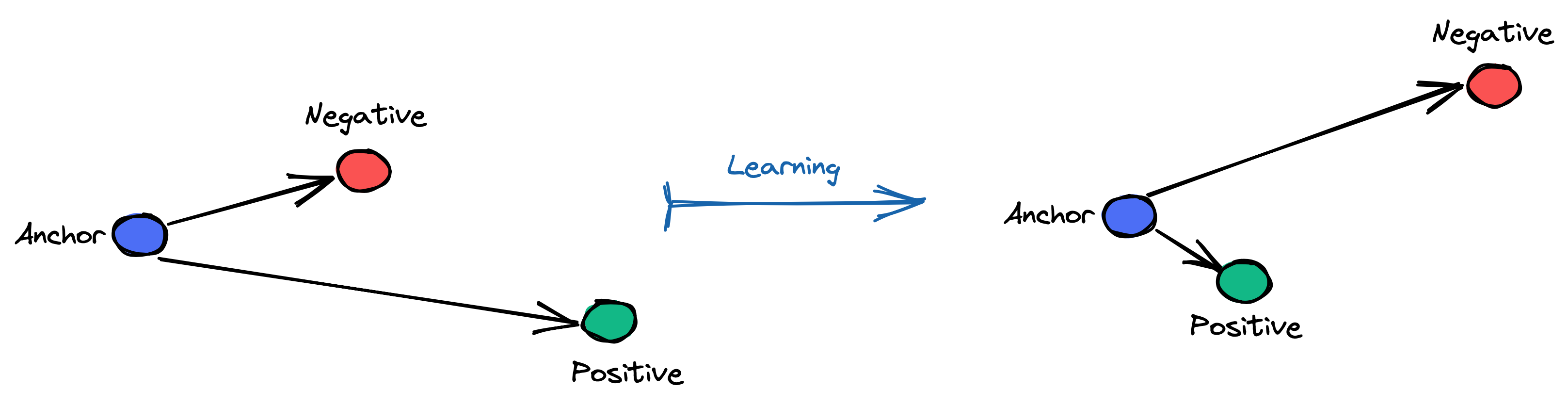
Triplet Loss is used for metric Learning, where a baseline (anchor) input is compared to a positive (truthy) input and a negative (falsy) input. The distance from the baseline (anchor) input to the positive (truthy) input is minimized, and the distance from the baseline (anchor) input to the negative (falsy) input is maximized
Consider the task of training a neural network to recognize faces (e.g. for admission to a high security zone). A classifier trained to classify an instance would have to be retrained every time a new person is added to the face database. This can be avoided by posing the problem as a similarity learning problem instead of a classification problem. Here the network is trained (using a contrastive loss) to output a distance which is small if the image belongs to a known person and large if the image belongs to an unknown person. However, if we want to output the closest images to a given image, we would like to learn a ranking and not just a similarity. A triplet loss is used in this case.
where, $a_i$ is the anchor, $p_i$ is the positive input, $n_i$ is the negative input and $d(x_i, y_i) = \Vert{x_i - y_i}\Vert_p$
Here's a figure depicting the objective we want to achieve during learning using Triplet Loss
triplet_loss = nn.TripletMarginLoss(margin=1.0, p=2)
anchor = torch.randn(100, 128, requires_grad=True)
positive = torch.randn(100, 128, requires_grad=True)
negative = torch.randn(100, 128, requires_grad=True)
output = triplet_loss(anchor, positive, negative)
output.backward()
Summary
We looked at different Loss functions in this multi-part series, this in no way was a comprehensive review of all the loss functions available, but instead just a brief overview of the most commonly used Loss functions. I'd encourage to read up on the different Loss functions available in PyTorch here.