Loss Functions Part 1
In this part of the multi-part series on Loss Functions we'll look at the concepts like Information Entropy, Cross Entropy, KL-Divergence, how they are linked to each other and how to code them in Python


Introduction
A Loss/Cost function or an objective function in Machine Learning (ML) is a function that maps the values of one or more variables to a scalar value. This scalar value is then used to minimize the loss/cost incurred while making a prediction. On a very high level, an ML algorithm works as follows:
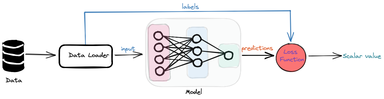
The diagram above is a very high-level overview of a model learning from data. We've simplified the training workflow a lot in the above diagram, we also have a step where the gradient of the loss wrt the model parameters gets calculated (we'll talk about autodiff in a detailed post later on) and then the optimizer uses those acumulated gradients for each parameter and updates the parameters for next iteration.
The choice of a loss function plays an important role in learning from data. It depends on what we want to learn, and what we want to predict. In some cases we just want to predict the distribution of the categories (discrete values), there we end up using a certain type of loss function while in some other cases we'd like to predict continuous values and there the choice of loss function would be completely different. Some time we'd like to perform metric learning, and the loss function for such a problem would not fall in the aforementioned categories. Below we review some of the loss functions that are most commonly used for some of the common problems in the field of ML.
Types of Loss Functions
Classification
Cross Entropy Loss
Entropy
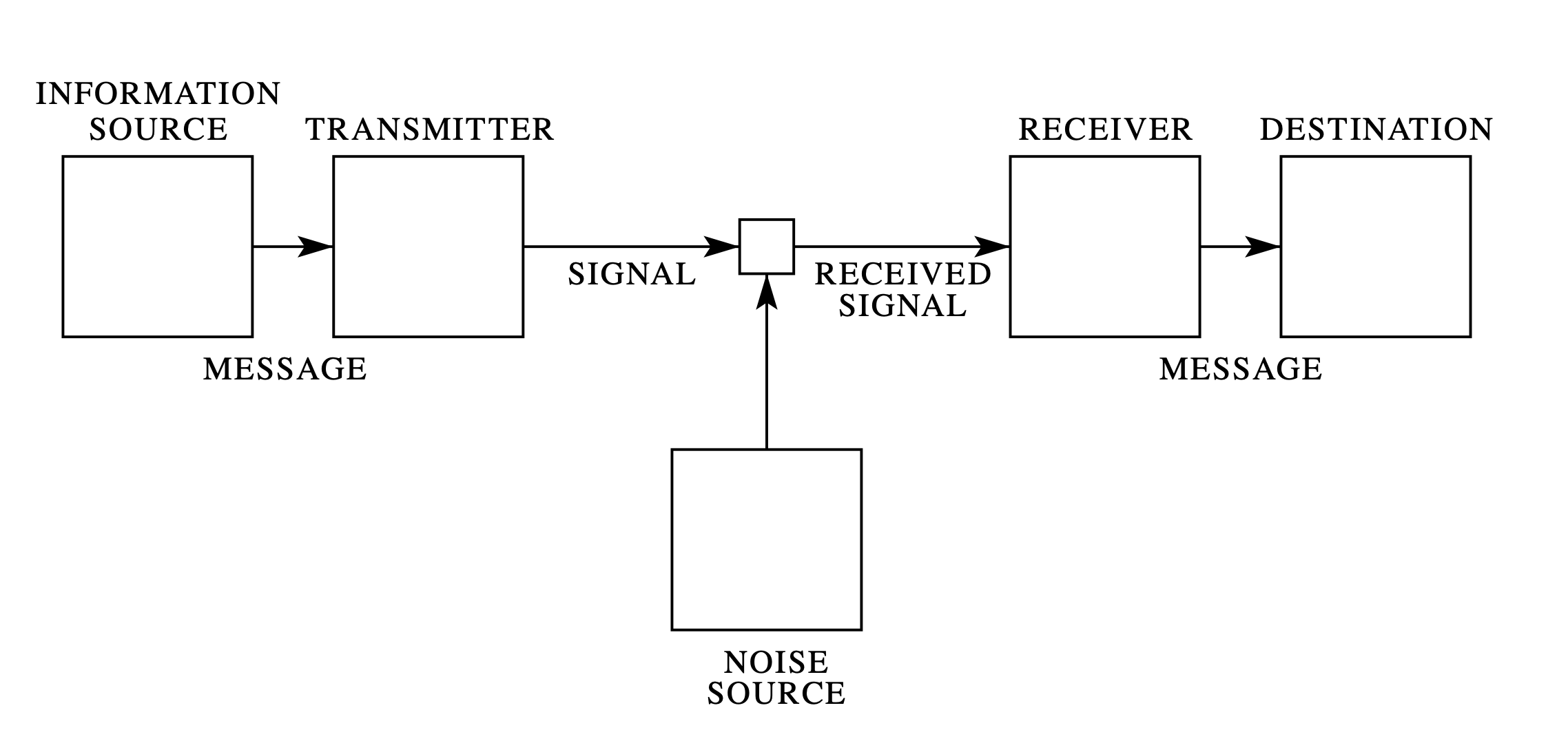
There's something to be said about Entropy before we look into Cross-Entropy. Entropy, is such a beautiful concept that I got first introduced to in an information theory course I took years ago. The whole process can be seen as how many bits we need to encode the message on the transmitter side to be able to successfully decode at the receiver. The concept was introduced by Claude Shannon and it is also known as Shannon entropy.
Formally, given a discrete random variable $X$, with possible outcomes $x_1,x_2,...,x_n$, which occur with probability $P(x_1),P(x_2),...,P(x_n)$ the entropy of $X$ is given by: $$ \boxed{H(X) = - \sum_{i=1}^{n} P(x_i) \log(P(x_i))} $$ What follows next is the characterization and can be found here on Wikipedia)
To understand the meaning of the above equation, first define an information function $I$ in terms of an event $x_i$ with probability $P(x_i)$. The amount of information acquired due to the observation of event $x_i$ follows from Shannon's solution of the fundamental properties of information.
- $I(p)$ is monotonically decreasing in $p$, an increase in the probability $p$ of an event decreases the information observed.
- $I(p) \geq 0$, information is a non-negative quantity
- $I(1) = 0$, events that always occur, don't convey any information
- $I(p_1, p_2)$ = $I(p_1) + I(p_2)$ if $p_1$ and $p_2$ are independent.
Shannon discovered that the suitable choice for $I$ is given by $I(p) = \log(p)$.
Using above to analyze the equation of $H(X)$, we see that the number of bits required to encode a message when $P(x_i) = 1$ or $P(x_i) = 0$ is $0$, this is due to the fact that we're either sure that the event will happen or it won't (we'll not communicate). An increase in the value of $P(x_i)$ decreases the value of the measure (Entropy).
Below is the plot of Information vs Probability or $I(p)$ vs $p$ which tells us that Information conveyed by the event decreases as Probability increases
from matplotlib import pyplot as plt
import numpy as np
import pandas as pd

from scipy.stats import norm
precision = 4
np.set_printoptions(precision=precision)
pd.set_option("precision", precision)
import torch
from torch.nn import functional as F

class InformationMeasure():
    @staticmethod
    def entropy(prob):
        return np.sum(-prob * np.log2(prob, out=np.zeros_like(prob), where=(prob!=0)))

class Plotter():
    @staticmethod
    def plot_xy(x,y, x_label, y_label, title, show_grid=True, legend=True,
                legend_loc='upper right', x_ticks=np.arange(0.0, 1.1, 0.5), plot_point=False, show_axes=True):
        with plt.xkcd():
            #plt.style.use('ggplot')
            fig, ax = plt.subplots(figsize=(8, 5))
            fig.tight_layout()
            ax.plot(x,y, linewidth=2.0, color='brown')
            if plot_point:
                ax.plot(0.5, 1.0, 'go', label='P(X = 1) = 0.5')
            ax.set_xlabel(x_label, fontsize=10,  color='black')
            ax.set_ylabel(y_label, fontsize=10,  color='black')
            ax.set_title(title, fontsize=15, color='black')
            ax.grid(False)
            if not show_axes:
                plt.axis('off')
            if legend:
                ax.legend(loc=legend_loc)
            x_ticks = ax.set_xticks(x_ticks)
            return fig, ax
class CoinToss():
    def __init__(self):
        self.x = np.arange(0.0, 1.0, 0.01)
        self.x = np.append(self.x, 1.0)
        self.hx = np.asarray([np.asarray(InformationMeasure.entropy(np.asarray(prob))) for \
                               prob in zip(self.x, 1-self.x)], dtype=np.float64)
    def plot(self):
        return Plotter.plot_xy(self.x, self.hx, x_label='P(X = 1)',
                               y_label='H(X)', title='Entropy of a coin flip',
                               plot_point=True)
class EntropyFunction():
    def __init__(self):
        self.x = np.arange(0.1, 1.0, 0.01)
        self.x = np.append(self.x, 1.0)
        self.hx = -np.log2(self.x, out=np.zeros_like(self.x), where=(self.x!=0))
    def plot(self):
        return Plotter.plot_xy(self.x, self.hx, x_label='$P(X)$',
                               y_label='$I(P(X))$',
                               title='Information vs Probability',
                               legend=False, x_ticks=np.arange(0.1, 1.1, 0.1))
entropy_func = EntropyFunction()
fig, ax = entropy_func.plot()

Now, let's consider as an example, tossing a biased coin whose probability of landing on heads is $p$ and the probability of landing on tails is $1-p$, this can be modelled as a Bernoulli Process. Below is the Entropy vs Probability plot for the process:
fig, ax = CoinToss().plot()

Cross-Entropy
Building upon the concept of Entropy we come across Cross-Entropy which tells us the average number of bits required to encode the information coming from a source distribution $P$ using a model distribution $Q$. $$ H(P, Q) = - \sum_{i=1}^{n} P(x_i) \log (Q(x_i)) $$ Here, we generally don't have access to the target distribution $P$, so we approximate it by the model distribution $Q$, and the closer $Q$ is to $P$ the lesser the average number of bits required to encode the information. One could also write $H(P,Q)$ in terms of expectation as follows: $$ H(P, Q) = - \mathbb{E}_{P(x)}[\log(Q(x))] $$
KL-Divergence
KL-Divergence (also known as relative entropy) is a type of f-divergence, which is a measure of how one probability distribution is different from the other. In Information theory terms, it's the extra number of bits required to encode the information from source distribution $P$ when using the model distribution $Q$. The divergence of $Q$ from $P$ is defined as: $$ \mathbb{D}_{KL}(P || Q) = \sum_{i=1}^{n} P(x_i) \log (\frac {Q(x_i)}{P(x_i)}) $$
Even though KL divergence is used to measure the distance between two distributions but it's a ditance metric. Some properties of KL Divergence are:
- It's not symmetric, i.e $\mathbb{D}_{KL}(P || Q) != \mathbb{D}_{KL}(Q || P)$
- It's non-negative, i.e $\mathbb{D}_{KL}(P || Q) >= 0$ and $\mathbb{D}_{KL}(P || Q) = 0$ only if $P = Q$
Some intuitions and explanations about KL Divergence:
-
If $P(x) = 0$ then during optimization it doesn't matter what the value of $Q(x)$ is as KL evaluates to 0. What this means is that when we don't have any weight in the source distribution but we do in target distribution, the target distribution is ignored.
-
If $P(x) > 0$, then we have a divergence, and if the modes of $Q(x)$ and $P(x)$ don't overlap then we'll incur a cost. The optimizer will then try to spread $Q(x)$ out so that the divergence is minimized.
Let's look at the graph below to make sense of what has been said in the two points above:

The figure above demonstrates the case where $P(x) > 0$ and $Q(x)$ doesn't match all the modes of the distribution, in this case KL Divergence will be high and the optimizer will try to move it $Q(x)$ such that it covers parts pf both the modes as shown below:

For this reason, this form of KL Divergence is known as zero-avoiding as it is avoiding $Q(x) = 0$ whenever $P(x) > 0$
There's one more form of KL Divergence as well, known as Reverse KL Divergence, that's something we'll cover when we talk about Variational Inference, the reason for that is that we need to talk about ELBO (Evidence Lower Bound)
Putting it all together
One can see that there exists a relationship between $\mathbb{D}_{KL}(P || Q)$ and $H(P,Q)$. Let's see if we can write one in terms of the other. $$ \mathbb{D}_{KL}(P || Q) = \sum_{i=1}^{n} P(x_i) \log (\frac {Q(x_i)}{P(x_i)}) \implies -\mathbb{E}_{P(x)}\left [log\left(\frac{Q(x)}{P(x)}\right)\right] \implies -\mathbb{E}_{P(x)}[\log(Q(x))] + \mathbb{E}_{P(x)}[\log(P(x))] $$
$$ \mathbb{D}_{KL}(P || Q) = -\mathbb{E}_{P(x)}[\log(Q(x))] + \mathbb{E}_{P(x)}[\log(P(x))] $$$$ \mathbb{D}_{KL}(P || Q) = H(P,Q) - H(P) \implies H(P,Q) = H(P) + \mathbb{D}_{KL}(P || Q) $$Calculating Cross Entropy and KL Divergence
The code for calculating Cross Entropy and KL Divergence is just the direct translation of the equations above.
In what follows next, we're assuming that the input to these functions are probability distributions.
def cross_entropy(p, q):
    # both p and q are asuumed be probability distributions.
    return np.sum(-p * np.log(q))
A way to turn scores into probability distribution is via Softmax function, which is defined as follows:
def softmax(p):
    return np.exp(p)/np.sum(np.exp(p), axis=-1, keepdims=True)
Notice how we're using the axis parameter to only take the sum along the last dimension in case we're dealing with more than one dimensions (which usually is the case).
Next, we'll create sample probability distributions for demonstration purposes.
def get_sample_dist(rs, size=(10,)):
    # Return a sample (or samples) from the "standard normal" distribution.
    scores = rs.randn(*size)
    # covert to a probability distribution
    p = softmax(scores)
    return scores, p
def sanity_check_dist(p):
    if p.ndim > 1:
        expected = np.ones(p.shape[-2])
    else:
        expected = 1.0
    return np.allclose(np.sum(p, axis=-1), expected)
def print_as_table(p):
    return pd.DataFrame(data=p, index=[f"{i}" for i in range(p.shape[0])], columns=[f"{i}" for i in range(p.shape[1])])
We'll now out to test what we've coded so far
seed = 42
rs = np.random.RandomState(seed)
scores_p, p = get_sample_dist(rs, (10,5))
scores_q, q = get_sample_dist(rs, (10,5))

sanity_check_dist(p), sanity_check_dist(q)
Here's how $p^*$ looks like:
$^*$For demonstration purposes, I've chosen the distributions to be 2 dimensional so that it can be visually inspected.
print_as_table(p)
Here's how $q$ looks like:
print_as_table(q)
print(f'Cross Entropy between P and Q: {cross_entropy(p,q): .4f}')
print(f'Cross Entropy between P and P: {cross_entropy(p,p): .4f}')
print(f'Entropy of P: {entropy(p): .4f}')
The code snippet calculates cross entropy, to calculate kl divergence we'll introduce another function
def kl_div(p, q):
    return np.sum(-p * (np.log(q) - np.log(p)))
print(f'KL Divergence of Q from P: {kl_div(p,q): .4f}')
To verify the relationship between Cross Entropy and Kl Divergence let's introduce another function to calculate entropy:
def entropy(p):
    return np.sum(-p * np.log(p))
np.allclose(kl_div(p,q) + entropy(p), cross_entropy(p,q))
Now, let's take a look at how the Cross Entropy Loss is implemented in a Machine Learning framework like PyTorch, from the PyTorch Documnetation about Cross Entropy Loss (also known as categorical cross entropy)
"This criterion combines LogSoftmax and NLLLoss in one single class. It is useful when training a classification problem with C classes."
So, it turns out, we only need to send in scores to this function as it combines LogSoftMax and NLLLoss. We also need to send in class labels to the function, effectively the function caluclates the following:
$$ loss(x, class) = - \log \left[ \frac{\exp(x[class])}{\sum_{j} x[j]}\right] \implies -x[class] + \log\left[ \sum_{j} \exp(x[j])\right] $$torch.manual_seed(42)
minibatch_size = 10
num_classes = 5
inputs = torch.randn(minibatch_size, num_classes)
targets = torch.empty(minibatch_size, dtype=torch.long).random_(num_classes)
loss = F.cross_entropy(inputs, targets)
loss
Let's use our inputs from before, remember that we have to send raw-scores and class labels. targets correspond to p and inputs correspond to scores_q
inputs = torch.from_numpy(scores_q)
targets = torch.from_numpy(np.argmax(p, axis=1))
loss = F.cross_entropy(inputs, targets)
loss
Notice how F.cross_entropy calculates the cross entropy between class labels and a probability distribution, that's the only difference (conceptually speaking) between the code we've written to calculate the the cross entropy and the PyTorch version
def cross_entropy_loss(inputs, targets):
    return np.asarray([np.mean(-np.take_along_axis(inputs, targets, 1) +
                                        np.log(np.sum(np.exp(inputs), axis=-1, keepdims=True)))])
There's another way to implement this function using for loops, but numpy broadcasting is much faster and we should always use that when we can
classes = np.expand_dims(np.argmax(p, axis=1), axis=1)
cross_entropy_loss(scores_q, classes)
Summary
We looked at the concepts like Entropy, Cross Entropy and KL Divergence from the point of view of Information Theory and got a sense of how to implement them and how they're implemented in a Deep Learning Framework like PyTorch, from here things should get a lot easier when we think about Cross Entropy and KL Divergence
I'll stop here for now and in the next post in the series about Loss Functions cover the following:
- MSE
- MAE
- Huber Loss
- Triplet Loss
- Hinge Loss
References
- A Mathematical Theory of Communication
- Cross Entropy Loss VS Log Loss VS Sum of Log Loss
- A Gentle Introduction to Cross-Entropy for Machine Learning
- nn.CrossEntropyLoss
- Lecture 2: Entropy and Data Compression (I): Introduction to Compression, Inf.Theory and Entropy, David MacKay, University of Cambridge
- Variational Inference
- KL Divergence Forward vs Reverse
- Overlapping probability of two normal distribution with scipy
- Notes on KL Divergence
- PyTorch Loss Functions: Ultimate Guide